

An output-ripple FFT is comparable only when the acquired time record, window, scaling and measurement conditions are known. A smoother spectrum or smaller displayed frequency increment does not, by itself, establish lower ripple or better separation of nearby components.
Key engineering takeaways
- Calculate acquired duration before interpreting frequency detail.
- Separate FFT grid spacing from window-dependent bandwidth.
- Keep voltage amplitude, spectral density and time-domain ripple distinct.
- Preserve the source waveform with every reported spectrum.
What should the spectrum help the OEM decide?
Use the FFT to investigate a defined question, such as whether two repeatable ripple components can be distinguished under a fixed load. An acceptance requirement for maximum time-domain peak-to-peak ripple remains a different question. Changing the display cannot make those two criteria interchangeable.
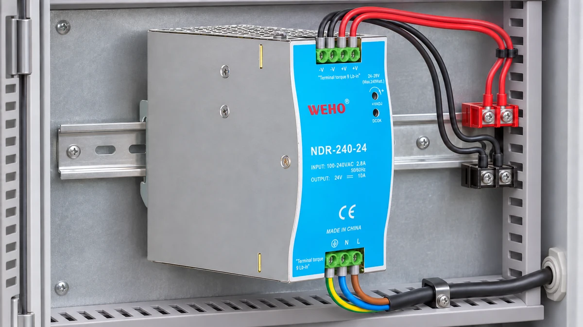
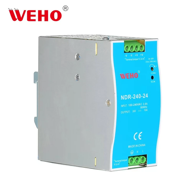
For an NDR-240-24 measurement review, identify the actual supply revision, receiver and measurement node. The product reference establishes the candidate being discussed. It does not establish switching frequency, a ripple spectrum or an instrument setting appropriate to every installation.
Keep the input condition, output load, local capacitance and harness configuration with the record. A trace captured during startup describes another operating state from a stabilized load. If the operating state changes inside the selected analysis interval, the spectrum can combine several behaviors that a single peak label conceals.
The existing power supply ripple acceptance guide addresses the voltage requirement and its measurement conditions. This article addresses what a finite-record FFT can support after an appropriate waveform has been acquired. Neither a spectral screenshot nor a catalog ripple number replaces the agreed equipment requirement.
Which time record actually enters the FFT?
For a uniformly sampled record containing N acquired samples at sampling rate fs, define the analysis duration as T = N/fs. Without zero padding, the FFT frequency-bin spacing is Δf = fs/N = 1/T. This duration convention describes the sampled block; the interval between the first and last sample timestamps is one sample interval shorter.
Keysight's FFT operator documentation explains that window choice changes the bandwidth associated with an FFT result. Therefore, write “100 Hz bin spacing” when that is what was calculated. Avoid replacing it with “100 Hz guaranteed resolving ability,” which also depends on the window, component amplitudes, noise and instrument behavior.
Check whether the instrument transforms the entire acquisition or a selected gate. A long stored acquisition can still produce a short analysis interval. Read the actual FFT input or gate settings instead of assuming that the oscilloscope's largest advertised memory depth was used for the displayed spectrum.
A hypothetical comparison of two nearby components
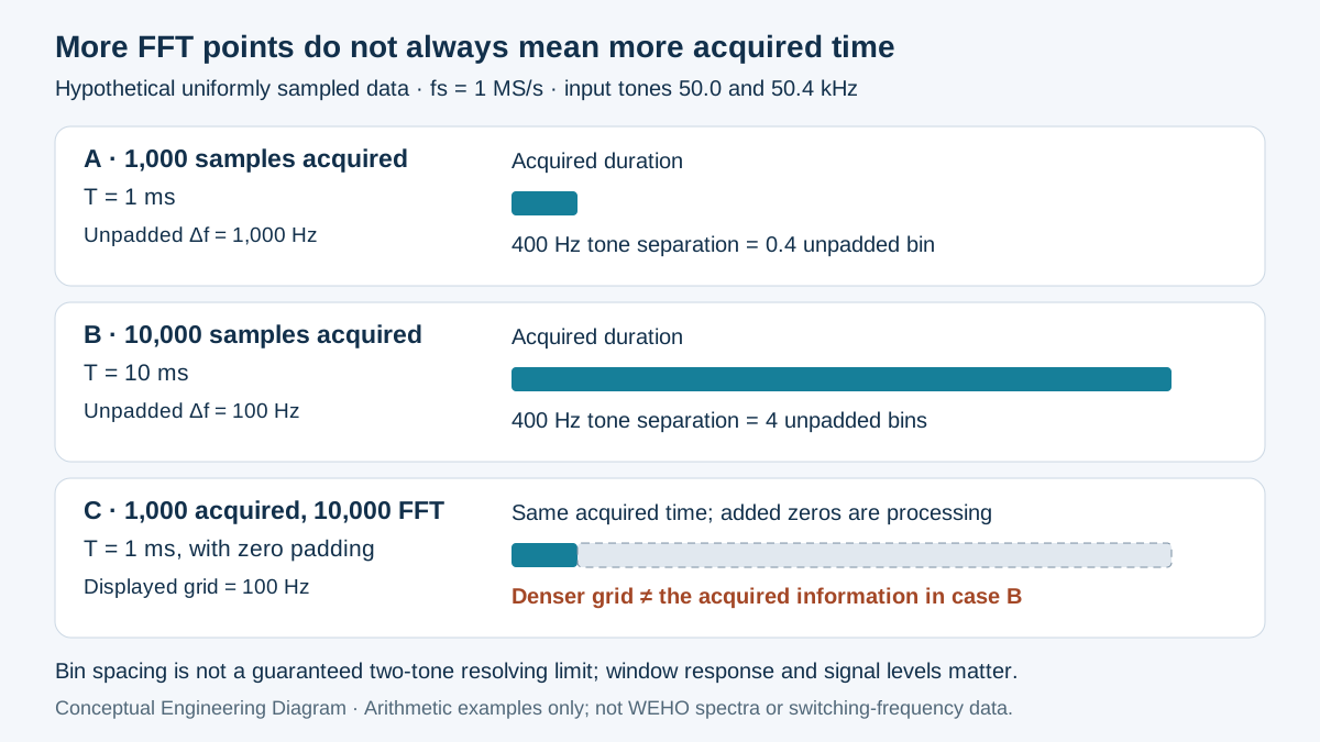
Assume an ideal sampled signal contains stable sinusoidal components at 50.0 kHz and 50.4 kHz. Their separation is 400 Hz. Assume a 1 MS/s acquisition rate, suitable analog measurement bandwidth and no aliasing within this illustrative comparison. These frequencies are invented signal inputs, not NDR-240-24 switching-frequency data or a measured WEHO waveform.
With 1,000 acquired samples, T = 1,000/1,000,000 = 0.001 s. The unpadded spacing is 1,000 Hz, so the 400 Hz separation spans only 0.4 bin. Reading extra digits from a peak marker cannot supply the missing acquired duration or establish that two independent components have been resolved.
With 10,000 acquired samples at the same rate, T = 0.010 s and the unpadded spacing becomes 100 Hz. The separation spans four bins. This is a more useful starting point for the comparison, but it remains necessary to examine the chosen window, relative component levels and the actual displayed response.
| Analysis case | Acquired samples | Acquired duration | FFT grid spacing |
|---|---|---|---|
| Short record, no padding | 1,000 | 1 ms | 1,000 Hz |
| Long record, no padding | 10,000 | 10 ms | 100 Hz |
| Short record padded to 10,000 points | 1,000 | 1 ms | 100 Hz display grid; original time support retained |
Swipe horizontally on a small screen, or open the full-size diagram.
The third row adds zero-valued samples computationally, rather than acquiring another nine milliseconds of signal. The resulting denser frequency grid can help display or interpolate the existing information. It does not provide the same independent resolving information as the genuinely longer acquisition in the second row.
Keysight's time-record explanation distinguishes acquired time length from FFT processing length. Record both when software pads data automatically. A reviewer needs to know which quantity changed before accepting a claim that a new screenshot reveals more physical frequency detail.
For an additional bandwidth check, assume the implementation uses a Hann window with normalized equivalent noise bandwidth of 1.5. Applying the documented time-to-bandwidth relationship, RBW = 1.5/T gives 150 Hz for the 10 ms record. This explicitly assumed implementation illustrates why the 100 Hz grid and 150 Hz noise bandwidth should occupy different fields; neither number is a universal two-tone separation criterion.
Choose the window for the measurement question
A finite record effectively joins its ending to its beginning when interpreted as a repeating block. A mismatch at that boundary can distribute a component's energy across neighboring frequencies. NI's FFT and windowing guidance describes this leakage and the tradeoff between suppressing sidelobes and widening the main response.
Select the comparison deliberately rather than cycling windows until the trace looks favorable. A nearby small component can be obscured by the response of a larger one. Conversely, a broad window response can make distinct components difficult to separate even when the plotted grid has many closely spaced points.
| Decision | Window consideration | Record to retain | Acceptance boundary |
|---|---|---|---|
| Investigate nearby components | Main-lobe width and sidelobes both matter | Window, duration, component levels and raw data | Demonstrate separation; do not infer it from grid spacing alone |
| Estimate an individual tone’s amplitude | Use the instrument’s documented amplitude correction and suitable window | RMS or peak convention and correction state | Compare like amplitude definitions |
| Compare broadband noise | Noise bandwidth and density scaling matter | Bandwidth, averaging and units | A lower per-bin level alone is insufficient |
| Capture a brief nonrepeating event | Preserve event timing and selected interval | Original waveform and gate position | Do not present an averaged spectrum as the complete event |
Identify whether the vertical axis reports volts, dBV or a density quantity. Do not read one spectral ordinate as total peak-to-peak ripple. Summation or integration requires the appropriate amplitude, window and bandwidth normalization; use the instrument's documented method rather than adding decibel values arithmetically.
Build a reproducible FFT comparison record
- Define the decision. Record the operating state, frequency region and whether the task concerns separation, tone amplitude or noise. Accept the plan only when the requested output can answer that question without substituting a different ripple criterion.
- Preserve the waveform. Record measurement node, probe arrangement, coupling, analog bandwidth, sample rate and acquired samples. Verify that the saved data contain the interval being analyzed and remain within the instrument's input limits.
- Calculate the duration. Record N, fs, selected gate and T. Recompute the unpadded spacing, identify any zero padding, and check that a claimed improvement follows from additional acquired information rather than a display setting alone.
- Fix the analysis conventions. Record the window, amplitude correction, vertical units and averaging. Verify that comparison files use the same conventions, or explain and validate each conversion before comparing their numerical levels.
- Test the interpretation. Repeat the relevant stable operating condition with an appropriate longer record or another justified window. Accept a frequency-detail claim only when the actual evidence supports it, while retaining inconclusive and changed-condition records.
Prepare an NDR-240-24 spectrum review
Send WEHO the NDR-240-24 source identity, actual input and load conditions, receiver requirement and the saved waveform. Include the FFT configuration and explain the engineering decision the spectrum should support. Request the applicable product documentation separately from any proposed test interpretation.
Before the next comparison, complete the duration calculation, record the window and units, and preserve the original data beside the screenshot. Those three actions make a spectrum reviewable without presenting a hypothetical signal, a product photograph or a favorable display as a completed product test.
Engineering FAQ
Does a 100 Hz FFT grid guarantee separation of two tones 100 Hz apart?
No. Grid spacing describes the computed frequency points, while practical separation also depends on the acquired duration, window response, relative amplitudes and noise. Record those conditions and examine the actual response before claiming that two components have been independently identified.
Does zero padding provide the information of a longer acquisition?
No. Zero padding adds processing points to the acquired block without observing additional signal time. A denser display can assist interpretation, but the record should retain the original acquired length so interpolation is not confused with new measurement information.
Can an FFT peak be compared directly with a peak-to-peak ripple limit?
No. A spectral component and a time-domain peak-to-peak result describe different quantities. Apply the specified ripple method and use spectral analysis to investigate relevant components; convert or combine quantities only through a justified, documented method.
Do the example frequencies specify the NDR-240-24 switching frequency?
No. The 50.0 kHz and 50.4 kHz components are hypothetical inputs used to explain finite-record analysis. Obtain exact-model information and actual appropriately acquired data before assigning a physical frequency component or test result to a WEHO supply.